Machine learning basics
1. Linear Regression with Multiple Variables
Table data example
A multifeature variable is a variable that stores several related characteristics about one item or subject, instead of just a single value. Like the example in this table:
| Size(feet2) | N bedrooms | N floors | Age | Price (1K) |
|---|---|---|---|---|
| x1 | X2 | X3 | X4 | y |
| 2104 | 5 | 1 | 45 | 460 |
| 1416 | 3 | 2 | 40 | 232 |
| 1534 | 3 | 2 | 30 | 315 |
| 852 | 2 | 1 | 36 | 178 |
| ... | ... | ... | ... | ... |
Naming Convention
When defining your feature matrix X:
- Always include a bias term:
X₀ = 1for all rows. - X₠… Xₙ → feature columns (n variables)
- m → number of training examples (rows)
- X11 … X1m → feature values per example
Equations
- Linear hypothesis
$$ h_\theta(x) = \theta^T x = \theta_0 x_0 + \theta_1 x_1 + \theta_2 x_2 + \cdots + \theta_n x_n $$
- Quadratic hypothesis (example of adding polynomial terms)
$$ h_\theta(x) = \theta_0 + \theta_1 x_1 + \theta_2 x_2 + \theta_3 x_1^2 + \theta_4 x_2^2 + \theta_5 x_1 x_2 + \cdots $$
- Cost function (least squares)
$$ J(\theta) = \frac{1}{2m} \sum_{i=1}^{m} \bigl(h_\theta(x^{(i)}) - y^{(i)}\bigr)^2 $$
- Gradient descent update
$$ \theta_j := \theta_j - \alpha\, \frac{1}{m} \sum_{i=1}^{m} \bigl(h_\theta(x^{(i)}) - y^{(i)}\bigr)\, x^{(i)}_j \quad \text{for } j=0,\dots,n $$
Example
-
Graphing the data
import pandas as pd
import numpy as np
import seaborn as sns
import matplotlib.pyplot as plt
pd.options.display.max_columns = 500
pd.options.display.max_rows = 500
# =============================================================================

#Load data
data = pd.read_csv(r'_data/ex1data1.txt', header=None, names=['x', 'y'])

#Plot data
plt.plot(data.x, data.y, 'o')
plt.title('Data points')
plt.xlabel('X axis')
plt.ylabel('Y axis')
plt.show()

#variables calculation
m = len(data.x)
theta = np.array([0, 0])
vector_x = np.array([[1]*len(data.x), data.x]).transpose()
vector_y = np.array(data.y)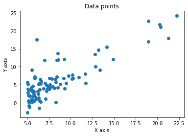
-
Initial cost function calculation
#Cost function calculation
def costfunc(vec_x, vec_y, theta, m):
    hypothesis = vec_x.dot(theta.transpose())
    error = (hypothesis-vec_y)
    cost = 1/(2*m) * np.sum(error**2)
    return cost, error

#output
cost = costfunc(vector_x,vector_y , theta, m)
print('The initial cost for theta {} is J = {}'.format(theta,cost[0]))
The initial cost for theta [0 0] is J = 32.072733877455676The cost value of 32.07 shows that the model’s predictions are still quite far from the actual data points.
This high error indicates that the initial parameters (θ = [0, 0]) need to be adjusted through training to better fit the data.
-
Gradient descent calculation
#Number of iterations
cycles = 200
alpha = 0.01

#Gradient descent
cost_h = []
for i in range(cycles):
    costf = costfunc(vector_x, vector_y, theta, m)
    cost = costf[0]
    cost_h.append(cost)
    error = costf[1]
    theta_0 = theta[0] - alpha*(1/m)*np.sum(error)
    theta_1 = theta[1] - alpha*(1/m)*np.sum(error*vector_x[:, 1])
    theta = np.array([theta_0, theta_1])

y_sol = [theta[0] + theta[1]*x for x in data.x]

#Plot cost function
print('Cost Function graph with Alpha = {} doing {} loops'.format(alpha, cycles))
f, axs = plt.subplots(1,2,figsize=(15,5))
plt.subplot(1, 2, 1)
plt.plot(list(range(cycles)), cost_h)
plt.xlabel('Number of Loops')
plt.ylabel('Error')

#Plot Line
plt.subplot(1, 2, 2)
plt.plot(data.x, y_sol, color = 'red')
plt.scatter(data.x, data.y,marker='x', s=20)


plt.show()
print()
print('The final error is {}'.format(cost))
print()
print('THE FINAL THETA IS {}'.format(theta))
Cost Function graph with Alpha = 0.01 doing 200 loops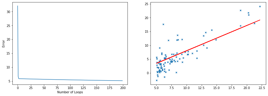
The final error is 5.1786804785845755

THE FINAL THETA IS [-1.12450181  0.9146286 ]
02. Logistic Regression Classification
Logistic Regression Classification is a method used to predict whether something belongs to one of two categories (like yes/no or 0/1).
It works by finding a relationship between the input features and the probability of an outcome using a special “S-shaped†curve called the sigmoid function.
Table data example
| Data | y | x1 | x2 | x3 | ... | x29 | x30 |
|---|---|---|---|---|---|---|---|
| Nº 1 | 0 | 1 | 0 | 1 | ... | 1 | 1 |
| Nº 2 | 1 | 0 | 0 | 0 | ... | 1 | 1 |
| Nº 3 | 0 | 0 | 0 | 1 | ... | 0 | 1 |
| ... | ... | ... | ... | ... | ... | ... | ... |
| Nº 599 | 1 | 0 | 1 | 0 | ... | 0 | 1 |
| Nº 600 | 1 | 1 | 0 | 1 | ... | 0 | 0 |
Equations
-
Sigmoid hypothesis
\[ h_\theta(x) = g(\theta^T x) = \frac{1}{1 + e^{-\theta^T x}} \\ h_\theta(x) = P(y = 1 \mid x; \theta) \]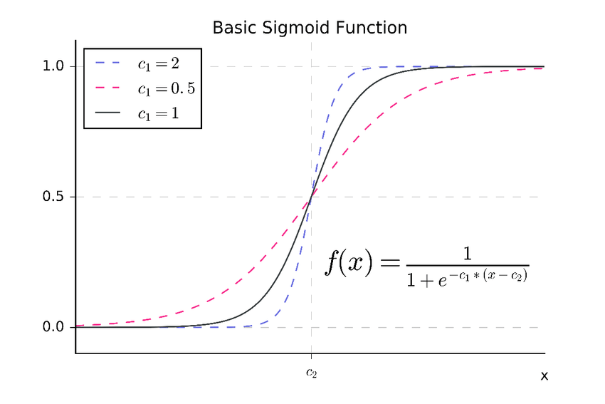 \[ g(z) \ge 0.5 \quad \text{when} \quad z(x) \ge 0 \]
 -
Non-linear decision boundaries
\[ h_\theta(x) = g(\theta_0 + \theta_1 x_1 + \theta_2 x_2 + \theta_3 x_1^2 + \theta_4 x_2^2) \] -
Cost function
\[ \text{cost}(h_\theta(x), y) = \begin{cases} -\log(h_\theta(x)), & \text{if } y = 1 \\ -\log(1 - h_\theta(x)), & \text{if } y = 0 \end{cases} \]\[ \text{cost}(h_\theta(x), y) = -y \log(h_\theta(x)) - (1 - y) \log(1 - h_\theta(x)) \]\[ J(\theta) = \frac{1}{m} \sum_{i=1}^{m} \text{Cost}(h_\theta(x^{(i)}), y^{(i)}) \]\[ J(\theta) = -\frac{1}{m} \left[ \sum_{i=1}^{m} y^{(i)} \log(h_\theta(x^{(i)})) + (1 - y^{(i)}) \log(1 - h_\theta(x^{(i)})) \right] \] -
Gradient descent
Gradient formula:
\[ \frac{\delta J(\theta)}{\delta \theta_j} = \frac{1}{m} \sum_{i=1}^{m} \left( h_\theta(x^{(i)}) - y^{(i)} \right) x_j^{(i)} \]Gradient descent:
\[ \min_{\theta} J(\theta) \]\[ \text{Repeat} \left\{ \theta_j := \theta_j - \alpha \frac{1}{m} \sum_{i=1}^{m} \left( h_\theta(x^{(i)}) - y^{(i)} \right) x_j^{(i)} \right\} \]
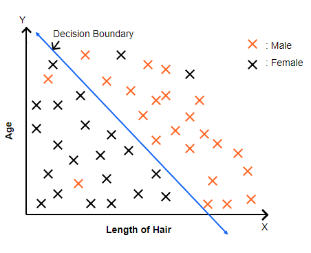
Decision boundary
This image shows how logistic regression divides data into two groups (Male and Female) using a decision boundary — the blue line.
Points on one side of the line are predicted as one class, and those on the other side as the opposite class; the line itself represents where the model is 50% unsure between the two.
Example
-
Graphing data
import pandas as pd
import numpy as np
import seaborn as sns
import matplotlib.pyplot as plt
pd.options.display.max_columns = 500
pd.options.display.max_rows = 500
# =============================================================================
# =========================== INSERT YOUR CODE BELOW ===========================
# =============================================================================

#Load data
data = pd.read_csv(r'_data\ex2data1.txt', header=None, names=['x', 'x1', 'y'])
datay0 = data.where(data.y == 0).dropna()
datay1 = data.where(data.y == 1).dropna()

#Printed data
print(data.head())

#Plot data
plt.scatter(datay0.x, datay0.x1, marker = 'x', color='red', label ='Not Admitted')
plt.scatter(datay1.x, datay1.x1, marker = 'o', color='green', label='Admitted')
plt.title('Second Exam')
plt.xlabel('First exam')
plt.ylabel('Y axis')
plt.legend()
plt.show()
x x1 y 0 34.623660 78.024693 0 1 30.286711 43.894998 0 2 35.847409 72.902198 0 3 60.182599 86.308552 1 4 79.032736 75.344376 1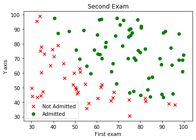
-
Initial cost function calculation
import math as mt

#variables calculation
m = len(data.x)
theta = np.zeros((3,1))
vector_x = np.array([[1]*len(data.x), data.x, data.x1]).transpose()
vector_y = np.array(data.y)[np.newaxis].T

#Cost function calculation
def sigmoid(lst):
    sigmoid = lambda x: 1/(1+mt.e**(-x))
    output = np.array([sigmoid(i) for i in lst])
    return output

def costfunc(vec_x, vec_y, theta, m):
    hx = vec_x.dot(theta)
    gx = sigmoid(hx)
    cost = vec_y * np.log(gx) + (1-vec_y) * np.log(1-gx)
    fcost = - (1/m) * np.sum(cost)
    return fcost, gx

#output
cost = costfunc(vector_x,vector_y , theta, m)
print('The initial cost for theta {} is J = {}'.format(theta.T,cost[0]))
The initial cost for theta [[0. 0. 0.]] is J = 0.6931471805599453 -
Gradient Descent
#Number of iterations
cycles = 5000
alpha = 0.001068
theta = np.array([-1, 0, 0])[np.newaxis].T

#Variables
cost_h = []
theta_0 = theta[0]
theta_1 = theta[1]
theta_2 = theta[2]

#Gradient descent
for i in range(cycles):
    cost = costfunc(vector_x, vector_y, theta, m)
    cost_h.append(cost[0])
    gx = cost[1]
    theta_0 = theta_0 - alpha * 1/m * np.sum((gx-vector_y)*vector_x[:, 0][np.newaxis].T)
    theta_1 = theta_1 - alpha * 1/m * np.sum((gx-vector_y)*vector_x[:, 1][np.newaxis].T)
    theta_2 = theta_2 - alpha * 1/m * np.sum((gx-vector_y)*vector_x[:, 2][np.newaxis].T)
    theta = np.array([theta_0, theta_1, theta_2])

#Otuput
print('The final error is {}'.format(cost_h[-3:]))
print()
print('THE FINAL THETA IS {}'.format(theta.T))
print()
print('The minimum error found with 300k cycles and alpha = 0.001068 is J = 0.27582976320910635')
print('And the final theta is: ')
theta = np.array([-9.78506335, 0.08377175, 0.0775022])[np.newaxis].T
print(theta.T)
The final error is [0.5451423473696985, 0.5451386883489806, 0.5451350293938765] THE FINAL THETA IS [[-1.31988582 0.0196853 0.01075302]] The minimum error found with 300k cycles and alpha = 0.001068 is J = 0.27582976320910635 And the final theta is: [[-9.78506335 0.08377175 0.0775022 ]] -
Algorithm trial
#Original hypothesis
eq = lambda x, y: sigmoid(theta[0] + x*theta[1] + y*theta[2])

#Select a point by index to know the y
index = 4
y = eq(vector_x[index, 1], vector_x[index, 2])

#Outputs
print('hypothesis theta = {}, {}, {}'.format(theta[0], theta[1], theta[2]))
print()
print('With this hypothesis the point P(x1, x2) = ({}, {}) would have a y = {}'.format(vector_x[index, 1], vector_x[index, 2], y))
hypothesis theta = [-9.78506335], [0.08377175], [0.0775022] With this hypothesis the point P(x1, x2) = (79.0327360507101, 75.3443764369103) would have a y = [0.93553537]#Resolving equation for two points theta.flatten() x_pts = [] y_pts = [] ##If x2 = 0 y_pts.append(0) x1 = -theta[0]/theta[1] x_pts.append(x1) ##If x1 = 0 x_pts.append(0) y2 = -theta[0]/theta[2] y_pts.append(y2) #Plot cost function print('Cost Function graph with Alpha = {} doing {} loops'.format(alpha, cycles)) f, axs = plt.subplots(1,2,figsize=(15,5)) plt.subplot(1, 2, 1) plt.plot(list(range(cycles)), cost_h) plt.xlabel('Number of Loops') plt.ylabel('Error') #Plot Line plt.subplot(1, 2, 2) plt.scatter(datay0.x, datay0.x1, marker = 'x', color='red', label ='Not Admitted') plt.scatter(datay1.x, datay1.x1, marker = 'o', color='green', label='Admitted') plt.plot(x_pts, y_pts) plt.title('Decision boundary test') plt.xlabel('First test') plt.ylabel('Second test') plt.legend() plt.show()Cost Function graph with Alpha = 0.001068 doing 5000 loops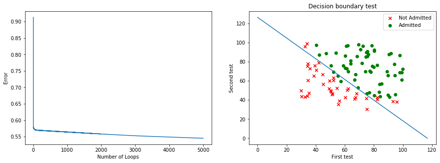
03. Neural Networks
Equations
Forward propagation
Hidden layer:
Output layer:
Cost function
Logistic regression regularization
Neural network regularization